Continuum Removal

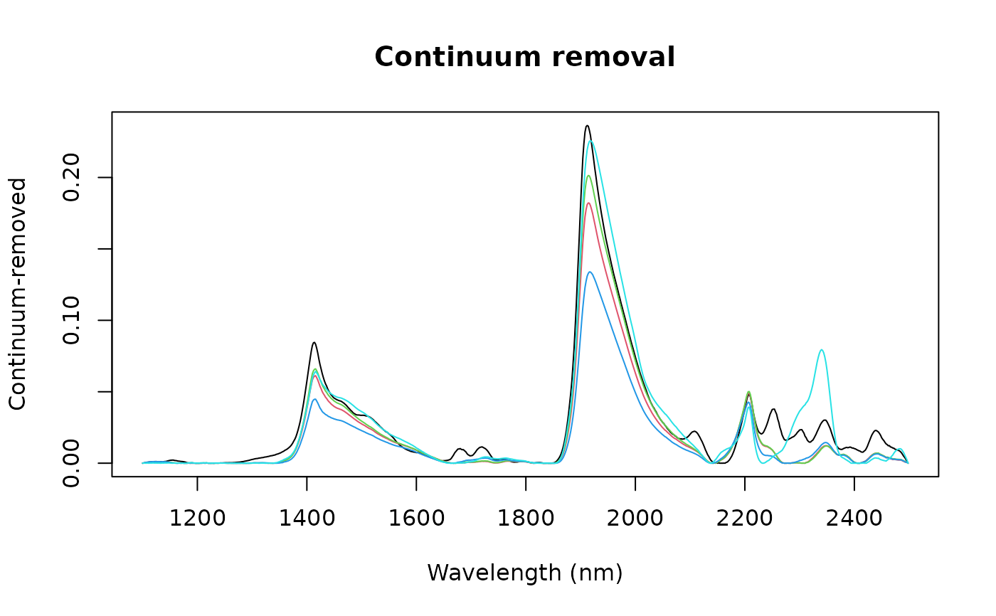
Compute the continuum-removed values of a data matrix or vector.

Usage

continuumRemoval(
  X, wav, type = c("R", "A"),
  interpol = c("linear", "spline"),
  method = c("division", "subtraction")
)

Arguments

X

a numeric matrix or vector to process (optionally a data frame that can be coerced to a numerical matrix).

wav

a numeric vector of band positions of length equal to ncol(X) (or length(X) if X is a vector). If not provided, integer indices 1:ncol(X) are used.

type

the type of data: "R" for reflectance (default), "A" for absorbance.

interpol

the interpolation method between convex hull points: "linear" (default) or "spline".

method

the normalisation method: "division" (default) or "subtraction" (see Details).

Value

a matrix or vector of continuum-removed spectra, with the same dimensions and dimnames as X.

Details

The continuum removal technique was introduced by Clark and Roush (1984) to highlight absorption features by removing the effect of the overall spectral shape (albedo). It is widely used in remote sensing and spectroscopy to isolate and compare absorption band depths across samples or sensors.

The algorithm identifies points lying on the convex hull (upper envelope) of a spectrum, connects them by linear or spline interpolation to form a continuum line, and normalises the spectrum against that line either by division or subtraction. Division (default, equivalent to the ENVI implementation) yields values in [0, 1] for reflectance spectra, where 1 indicates no absorption relative to the continuum. Subtraction yields residuals relative to the continuum (\(1 + x_i - c_i\)).

When type = "A" (absorbance), spectra are first converted to reflectance (\(1/X\)) before computing the convex-hull continuum, and the result is back-transformed to absorbance afterwards. This means that for absorbance data, continuumRemoval and baseline are not equivalent: they compute the convex hull on different scales (reflectance vs absorbance). For reflectance data (type = "R"), the two functions are more directly comparable, differing only in the final normalisation step: baseline subtracts the continuum (\(x_i - c_i\)), whereas continuumRemoval divides by it (\(x_i / c_i\)).

At wavelengths where both the spectral value and the continuum are zero, the continuum-removed value is set to 1 (no absorption feature), since division of zero by zero is undefined.

References

Clark, R.N., and Roush, T.L., 1984. Reflectance Spectroscopy: Quantitative Analysis Techniques for Remote Sensing Applications. J. Geophys. Res. 89, 6329–6340.

See also

baseline for a closely related method that subtracts the convex-hull envelope rather than dividing by it. savitzkyGolay, movav, gapDer, binning

Author

Antoine Stevens & Leonardo Ramirez-Lopez

Examples

data(NIRsoil)
wav <- as.numeric(colnames(NIRsoil$spc))
cr <- continuumRemoval(NIRsoil$spc, wav, type = "A")
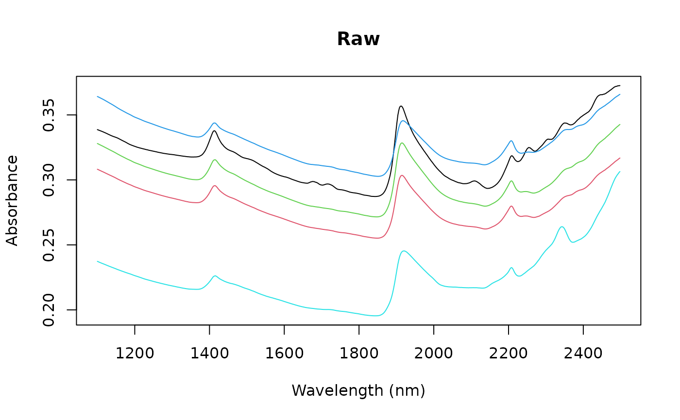
matplot(wav, t(NIRsoil$spc[1:5, ]),
  type = "l", lty = 1,
  xlab = "Wavelength (nm)", ylab = "Absorbance",
  main = "Raw"
)

matplot(wav, t(cr[1:5, ]),
  type = "l", lty = 1,
  xlab = "Wavelength (nm)", ylab = "Continuum-removed",
  main = "Continuum removal"
)