Building a library of models with liblex

Leonardo Ramirez-Lopez

2026-04-21

All models are wrong, but some are useful – (Box, 1976)

1 Introduction

Traditional memory-based learning (MBL) methods fit a new local model for each query observation. While effective, this per-query refitting can be computationally expensive and requires access to the full reference library at prediction time.

The liblex() function (library of localised experts) takes a different approach: it pre-computes a library of local models during a build phase, then retrieves and combines relevant experts at prediction time without refitting. This design offers several advantages:

• Computational efficiency: Models are fitted once; prediction requires only retrieval and weighted averaging.
• Privacy preservation: Only model coefficients and centroids need to be stored (not the original training spectra).
• Intrinsic uncertainty: Disagreement among retrieved experts provides a natural measure of prediction uncertainty.
• Interpretability: Each expert retains its regression coefficients and variable importance, enabling inspection of local relationships.

The method is introduced and described in detail in Ramirez-Lopez et al. (2026).

2 How liblex works

The liblex algorithm operates in two phases:

2.1 Build phase

1. Anchor selection: A subset of reference observations (anchors) is selected. Each anchor will generate one local expert model. By default, all observations serve as anchors; for large datasets, a representative subset can be specified via anchor_indices.

2. Neighborhood construction: For each anchor, the $k$ nearest neighbors are identified from the full reference set using a dissimilarity measure. Note that neighbors are drawn from all reference observations, not just anchors.

3. Local model fitting: A partial least squares (PLS) regression model (or variant such as weigthed average PLS or modified PLS) is fitted within each neighborhood, producing regression coefficients. The neighborhood centroid is stored for use during prediction.

4. Validation (optional): Nearest-neighbor cross-validation assesses performance and optimizes hyperparameters ($k$ and PLS component range).

2.2 Prediction phase

1. Expert retrieval: For a new observation, dissimilarities to all stored centroids are computed, and the $k$ nearest experts are retrieved. The same optimal $k$ determined during fitting is used here, so the number of anchors should be at least as large as the maximum $k$ being evaluated.

2. Weighted combination: Each retrieved expert generates a prediction. These predictions are combined via distance-based kernel weighting, with closer experts receiving higher weights.

3. Uncertainty estimation: The weighted variance across expert predictions provides a per-sample uncertainty estimate, reflecting disagreement among retrieved experts.

3 Data preparation

library(resemble)
library(prospectr)

data(NIRsoil)

# Wavelengths
wavs <- as.numeric(colnames(NIRsoil$spc))

# Preprocess: detrend + first derivative
NIRsoil$spc_pr <- savitzkyGolay(
  detrend(NIRsoil$spc, wav = wavs),
  m = 1, p = 1, w = 7
)

# Split into training and test sets
# Note: missing values in the response are allowed in liblex
train_x <- NIRsoil$spc_pr[NIRsoil$train == 1, ]
train_y <- NIRsoil$Ciso[NIRsoil$train == 1]
test_x  <- NIRsoil$spc_pr[NIRsoil$train == 0, ]
test_y  <- NIRsoil$Ciso[NIRsoil$train == 0]

cat("Training set:", nrow(train_x), "observations\n")

Training set: 618 observations

cat("Test set:", nrow(test_x), "observations\n")

Test set: 207 observations

4 Core components

4.1 Neighbor selection

Neighborhood size is specified using neighbors_k() for fixed-$k$ selection or neighbors_diss() for threshold-based selection. Multiple values can be provided for hyperparameter tuning.

# Fixed neighborhood sizes to evaluate
neighbors_k(k = seq(40, 120, by = 20))

Neighbor selection: fixed k
  k : 40, 60, 80, 100, 120 

# Threshold-based selection with bounds
neighbors_diss(
  threshold = seq(0.05, 0.5, length.out = 10), 
  k_min = 40, 
  k_max = 150
)

Neighbor selection: dissimilarity threshold
   threshold : 0.05, 0.1, 0.15, ..., 0.45, 0.5
   k_min     : 40
   k_max     : 150 

4.2 Dissimilarity methods

The dissimilarity measure determines how neighbors are identified. Available methods include diss_pca(), diss_pls(), diss_correlation(), diss_cosine(), etc (see the dissimilarity() function for all methods). The moving-window correlation dissimilarity is particularly effective for spectral data:

# Moving-window correlation dissimilarity (recommended for spectra)
diss_correlation(ws = 37, scale = TRUE)

Dissimilarity method: correlation
   window size (ws) : 37
   center           : TRUE
   scale            : TRUE 

# PCA-based Mahalanobis distance with optimized components
diss_pca()

Dissimilarity: PCA
  method            : pca
  ncomp             : var >= 0.01 (max: 40)
  center            : TRUE
  scale             : FALSE
  return_projection : FALSE 

4.3 Fitting method

The default method in the liblex() function to fit the local regressions is the weighted average PLS (waPLS), which combines predictions from multiple PLS component counts. The fit_wapls() constructor specifies the component range and algorithm:

# waPLS with modified PLS algorithm and scaling
fit_wapls(
  min_ncomp = 3, 
  max_ncomp = 15, 
  scale = TRUE, 
  method = "mpls"
)

Fitting method: wapls
   min_ncomp : 3
   max_ncomp : 15
   method    : mpls
   scale     : TRUE
   max_iter  : 100
   tol       : 1e-06 

4.4 Control parameters

The liblex_control() function specifies operational settings:

Parameter	Description
mode	"build" (fit models) or "validate" (evaluate only)
tune	If TRUE, optimize hyperparameters via nearest-neighbor validation
metric	Optimization metric: "rmse" or "r2"
allow_parallel	Enable parallel computation

# Build library with hyperparameter tuning
liblex_control(mode = "build", tune = TRUE)

5 Building a library of models

5.1 Using fixed neighborhood size(s)

The following example builds a library using fixed-$k$ neighbor selection with moving-window correlation dissimilarity:

ciso_lib_k <- liblex(
  Xr = train_x, 
  Yr = train_y, 
  neighbors = neighbors_k(seq(40, 80, by = 20)),
  diss_method = diss_correlation(ws = 37, scale = TRUE),
  fit_method = fit_wapls(
    min_ncomp = 3,
    max_ncomp = 15,
    scale = TRUE,
    method = "mpls"
  ),
  control = liblex_control(tune = TRUE)
)

ciso_lib_k

--- liblex model library ---
Models:     618
Predictors: 694
_______________________________________________________
Dissimilarity
Dissimilarity method: correlation
   window size (ws) : 37
   center           : TRUE
   scale            : TRUE
_______________________________________________________
Local fit method
Fitting method: wapls
   min_ncomp : 3
   max_ncomp : 15
   method    : mpls
   scale     : TRUE
   max_iter  : 100
   tol       : 1e-06
_______________________________________________________
Optimal parameters
  k:     40
  ncomp: 3 - 15
_______________________________________________________
Nearest-neighbor validation

Best results per neighbor selection metric
  k min_ncomp max_ncomp    r2  rmse      me st_rmse
 40         3        15 0.841 0.774 -0.1220   0.729
 60        10        10 0.784 0.897 -0.0763   0.696
 80         3        15 0.750 0.952 -0.1100   0.635
_______________________________________________________ 

The plot method for liblex objects visualizes the performance of the fitted experts across different neighborhood sizes and shows the centroids of the neighborhoods. Figure 1 shows the resulting plots for the library built with fixed neighborhood sizes. The top panel compares the performance of the best model obtained for each neighborhood size based on the RMSE, while the bottom panel displays the centroids of the neighborhoods, which are used later in prediction to select the models to be used.

plot(ciso_lib_k)

Figure 1: Top: Best model obtained for each neighborhood size (based on the RMSE). Bottom: Centroids of the neighborhoods, usled later in prediction to selet the models to be used.

The centroids in Figure 1 represent the average spectra of the neighbors for each expert. During prediction, the similarity between the new observation and these centroids is used to determine which experts to retrieve and how to weight their predictions.

5.2 Using dissimilarity thresholds

Alternatively, neighbors can be selected based on a dissimilarity threshold. The k_min and k_max arguments ensure reasonable neighborhood sizes:

--- liblex model library ---
Models:     618
Predictors: 694
_______________________________________________________
Dissimilarity
Dissimilarity method: correlation
   window size (ws) : 37
   center           : TRUE
   scale            : TRUE
_______________________________________________________
Local fit method
Fitting method: wapls
   min_ncomp : 3
   max_ncomp : 15
   method    : mpls
   scale     : TRUE
   max_iter  : 100
   tol       : 1e-06
_______________________________________________________
Optimal parameters
  diss threshold:     0.05
  ncomp: 3 - 15
_______________________________________________________
Nearest-neighbor validation

Best results per neighbor selection metric
 diss_threshold min_ncomp max_ncomp k_min k_max    r2  rmse      me st_rmse
          0.050         3        15    40   150 0.841 0.774 -0.1220   0.729
          0.162         3        15    40   150 0.841 0.775 -0.1280   0.696
          0.275         4        15    40   150 0.779 0.895 -0.1210   0.638
          0.388         5        15    40   150 0.751 0.933 -0.0812   0.610
          0.500        11        15    40   150 0.756 0.924 -0.0389   0.593
_______________________________________________________ 

ciso_lib_thr <- liblex(
  Xr = train_x, 
  Yr = train_y, 
  neighbors = neighbors_diss(
    threshold = seq(0.05, 0.5, length.out = 5), 
    k_min = 40, 
    k_max = 150
  ),
  diss_method = diss_correlation(ws = 37, scale = TRUE),
  fit_method = fit_wapls(
    min_ncomp = 3,
    max_ncomp = 15,
    scale = TRUE,
    method = "mpls"
  ),
  control = liblex_control(tune = TRUE)
)

ciso_lib_thr

5.3 Visualizing neighborhood centroids

The stored neighborhood centroids can be compared against the spectra to be predicted. Good coverage of the prediction space by the centroids indicates that relevant experts are available:

wavs_pr <- as.numeric(colnames(ciso_lib_k$scaling$local_x_center))

matplot(
  wavs_pr,
  t(test_x),
  col = rgb(1, 0, 0, 0.3),
  lty = 1,
  type = "l",
  xlab = "Wavelength (nm)",
  ylab = "First derivative detrended absorbance"
)

matlines(
  wavs_pr,
  t(ciso_lib_k$scaling$local_x_center),
  col = rgb(0, 0, 1, 0.3),
  lty = 1
)

grid(lty = 1)

legend(
  "topright",
  legend = c("Samples to predict", "Neighborhood centroids"),
  col = c(rgb(1, 0, 0, 0.8), rgb(0, 0, 1, 0.8)),
  lty = 1,
  lwd = 2,
  bty = "n"
)

Figure 2: Neighborhood centroids (blue) compared to test spectra (red)

5.4 Visualizing the regression models

The stored regression coefficients provide insight into how different spectral regions contribute to predictions across the library. Each expert model has its own set of coefficients, reflecting the local relationships learned within its neighborhood. Figure 3 shows an example of how the regression models can be visualized.

par(mfrow = c(2, 1), mar = c(4, 4, 2, 1))

# Regression coefficients across wavelengths
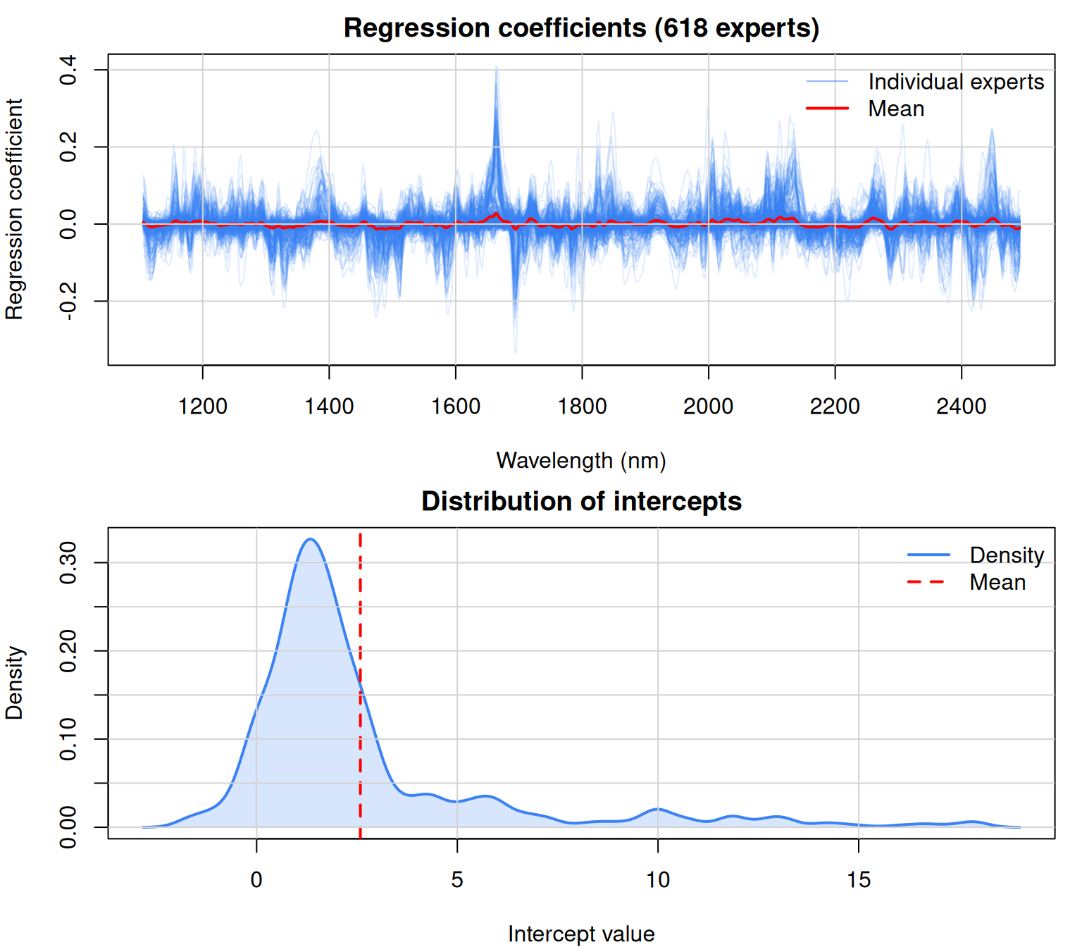
models <- ciso_lib_k$coefficients

matplot(
  x = wavs_pr,
  y = t(models$B),
  type = "l",
  lty = 1,
  col = rgb(0.23, 0.51, 0.96, 0.15),
  xlab = "Wavelength (nm)",
  ylab = "Regression coefficient",
  main = paste0("Regression coefficients (", nrow(models$B), " experts)")
)

# Add mean coefficient profile
lines(wavs_pr, colMeans(models$B), col = "red", lwd = 2)
grid(lty = 1)
legend(
  "topright",
  legend = c("Individual experts", "Mean"),
  col = c(rgb(0.23, 0.51, 0.96, 0.6), "red"),
  lty = 1,
  lwd = c(1, 2),
  bty = "n"
)

# Distribution of intercepts
plot(
  density(models$B0, na.rm = TRUE),
  col = rgb(0.23, 0.51, 0.96),
  lwd = 2,
  xlab = "Intercept value",
  ylab = "Density",
  main = "Distribution of intercepts"
)
polygon(
  density(models$B0, na.rm = TRUE),
  col = rgb(0.23, 0.51, 0.96, 0.2),
  border = NA
)
abline(v = mean(models$B0, na.rm = TRUE), col = "red", lty = 2, lwd = 2)
grid(lty = 1)
legend(
  "topright",
  legend = c("Density", "Mean"),
  col = c(rgb(0.23, 0.51, 0.96), "red"),
  lty = c(1, 2),
  lwd = 2,
  bty = "n"
)

par(mfrow = c(1, 1))

Figure 3: Regression coefficients (top) and intercept distribution (bottom) of the local experts

The top panel shows regression coefficients for each expert model across the spectral range, with the mean profile highlighted in red. Regions with high coefficient variability indicate wavelengths where local relationships differ substantially across the reference set. The bottom panel shows the distribution of intercepts, reflecting the range of baseline predictions across experts.

6 Choosing anchor samples

For large libraries, building models for every observation may be computationally prohibitive. The anchor_indices argument allows specifying a subset of observations as anchors while still using the full library for neighbor retrieval.

6.1 Using k-means sampling

The naes() function from the prospectr package implements the k-means sampling algorithm, which is a reasonable approach for selecting representative anchor samples:

# Select 350 representative anchors using k-means sampling
# on the first 20 principal components
set.seed(1124)
kms <- naes(
  train_x, 
  k = 350, 
  pc = 20, 
  iter.max = 100,
  .center = TRUE, 
  .scale = TRUE
)

anchor_km <- kms$model

cat("Selected", length(anchor_km), "anchors via k-means\n")

Selected 350 anchors via k-means

6.2 Building the library with selected anchors

--- liblex model library ---
Models:     350
Predictors: 694
_______________________________________________________
Dissimilarity
Dissimilarity method: correlation
   window size (ws) : 37
   center           : TRUE
   scale            : TRUE
_______________________________________________________
Local fit method
Fitting method: wapls
   min_ncomp : 3
   max_ncomp : 15
   method    : mpls
   scale     : TRUE
   max_iter  : 100
   tol       : 1e-06
_______________________________________________________
Optimal parameters
  k:     40
  ncomp: 3 - 15
_______________________________________________________
Nearest-neighbor validation

Best results per neighbor selection metric
  k min_ncomp max_ncomp    r2  rmse     me st_rmse
 40         3        15 0.817 0.861 -0.194   0.799
 60        10        10 0.776 0.937 -0.132   0.717
 80         3        15 0.727 1.020 -0.178   0.644
_______________________________________________________ 

ciso_lib_anchored <- liblex(
  Xr = train_x, 
  Yr = train_y, 
  neighbors = neighbors_k(seq(40, 80, by = 20)),
  diss_method = diss_correlation(ws = 37, scale = TRUE),
  fit_method = fit_wapls(
    min_ncomp = 3,
    max_ncomp = 15,
    scale = TRUE,
    method = "mpls"
  ),
  anchor_indices = anchor_km,
  control = liblex_control(tune = TRUE)
)

ciso_lib_anchored

the final number of models here can be verifyied by looking at the number of rows in the ciso_lib_anchored$coefficients$B matrix, which contains regression coefficients for each expert.

# Number of experts in the anchored library
n_experts <- nrow(ciso_lib_anchored$coefficients$B)
cat("Number of experts in the anchored library:", n_experts, "\n")

Number of experts in the anchored library: 350 

Is good practice to compare the spectra of the samples to be predicted against the centroids of the models stored in the library. Figure 4 shows the centroids of the anchored library compared to the test spectra. This visualization helps assess whether the selected anchors provide good coverage of the spectral space of the test samples, which is crucial for reliable predictions.

wavs_pr <- as.numeric(colnames(ciso_lib_anchored$scaling$local_x_center))
n_experts <- nrow(ciso_lib_anchored$scaling$local_x_center)
n_test <- nrow(test_x)

# Plot test spectra first (background)
matplot(
  wavs_pr,
  t(test_x),
  col = rgb(0.8, 0.2, 0.2, 0.2),
  lty = 1,
  type = "l",
  xlab = "Wavelength (nm)",
  ylab = "First derivative detrended absorbance",
  main = paste0("Coverage: ", n_experts, " experts vs ", n_test, " test samples")
)

# Overlay centroids
matlines(
  wavs_pr,
  t(ciso_lib_anchored$scaling$local_x_center),
  col = rgb(0.23, 0.51, 0.96, 0.3),
  lty = 1
)
grid(lty = 1)

legend(
  "topright",
  legend = c(
    paste0("Test samples (n = ", n_test, ")"),
    paste0("Centroids (n = ", n_experts, ")")
  ),
  col = c(
    rgb(0.8, 0.2, 0.2, 0.5),
    rgb(0.23, 0.51, 0.96, 0.5)
  ),
  lty = 1,
  lwd = c(1, 1, 2, 2),
  bty = "n"
)

Figure 4: Neighborhood centroids from anchored library compared to test spectra

7 Prediction

The predict() method retrieves relevant experts for each new observation and combines their predictions:

ciso_pred <- predict(ciso_lib_k, newdata = test_x, verbose = FALSE)

# Prediction output structure
names(ciso_pred)

[1] "predictions"        "neighbors"          "expert_predictions"

# Main predictions with uncertainty
head(ciso_pred$predictions)

         pred    pred_sd          q5       q25       q50       q75       q95
619 0.3856244 0.19534744  0.06028928 0.2479403 0.4291209 0.4855056 0.7145855
620 0.6936664 0.70140718 -1.95561730 0.9527322 0.9787370 0.9853943 1.1206657
621 1.1331650 0.18555775  0.81484841 1.0048035 1.1124210 1.2856018 1.4211193
622 1.4141111 0.06891127  1.29355804 1.3610080 1.4031863 1.4623839 1.5159899
623 0.8500144 0.05597980  0.76986805 0.8140432 0.8614580 0.8834105 0.8858314
624 1.3267730 0.24224839  0.92933949 1.1718196 1.3035218 1.4743276 1.6997474
           gh min_yr max_yr below_min above_max
619 2.3028909  0.100  2.551     FALSE     FALSE
620 0.5641504  0.190 10.856     FALSE     FALSE
621 0.3717648  0.763  5.034     FALSE     FALSE
622 0.3241581  0.890  2.230     FALSE     FALSE
623 1.1158321  0.643  3.468     FALSE     FALSE
624 0.4121674  0.753  3.869     FALSE     FALSE

7.1 Prediction output

The prediction result contains:

Component	Description
pred	Weighted mean prediction
pred_sd	Weighted standard deviation (uncertainty proxy)
pred_q*	Weighted quantiles of expert predictions
gh	GH distance (Mahalanobis distance in PLS space)
min_yr, max_yr	Response range in the neighborhood
below_min, above_max	Flags for extrapolation

7.2 Weighting options

The weighting argument controls how expert predictions are combined:

# Gaussian kernel (default)
predict(ciso_lib_k, newdata = test_x, weighting = "gaussian")

# Tricubic kernel (similar to LOCAL algorithm)
predict(ciso_lib_k, newdata = test_x, weighting = "tricube")

# Equal weights
predict(ciso_lib_k, newdata = test_x, weighting = "none")

Available kernels include "gaussian", "tricube", "triweight", "triangular", "quartic", "parabolic", and "cauchy".

7.3 Enforcing specific experts

The enforce_indices argument ensures certain experts are always included in the prediction neighborhood. This is useful when some anchors are known to be from the same domain as the target observations.

# Always include specific experts in predictions
predict(ciso_lib_k, newdata = test_x, enforce_indices = c(1, 5, 10))

8 Validation and performance

8.1 Evaluation metrics

pred_values <- ciso_pred$predictions$pred
pred_sd <- ciso_pred$predictions$pred_sd

# Performance metrics (excluding missing values)
complete <- !is.na(test_y)
r2 <- cor(pred_values[complete], test_y[complete])^2
rmse <- sqrt(mean((pred_values[complete] - test_y[complete])^2))

cat("R²:  ", round(r2, 3), "\n")

R²:   0.903 

cat("RMSE:", round(rmse, 3), "\n")

RMSE: 0.514 

8.2 Uncertainty as a quality filter

The prediction standard deviation (pred_sd) reflects disagreement among experts and can be used to identify unreliable predictions:

# Filter predictions by uncertainty threshold
unc_threshold <- quantile(pred_sd[complete], 0.75)
reliable <- complete & (pred_sd < unc_threshold)

r2_filtered <- cor(pred_values[reliable], test_y[reliable])^2
rmse_filtered <- sqrt(mean((pred_values[reliable] - test_y[reliable])^2))

cat("After filtering high-uncertainty predictions:\n")

After filtering high-uncertainty predictions:

cat("  Retained:", sum(reliable), "/", sum(complete), "observations\n")

  Retained: 138 / 184 observations

cat("  R²:      ", round(r2_filtered, 3), "\n")

  R²:       0.936 

cat("  RMSE:    ", round(rmse_filtered, 3), "\n")

  RMSE:     0.19 

8.3 Visualization

lims <- range(pred_values[complete], test_y[complete], na.rm = TRUE)

plot(
  pred_values[complete],
  test_y[complete],
  pch = 16,
  col = rgb(0, 0, 0, 0.5),
  xlab = "Predicted",
  ylab = "Observed",
  xlim = lims,
  ylim = lims
)

abline(0, 1, col = "red", lwd = 2)
grid(lty = 1)

Figure 5: Predicted versus observed values

9 Comparison with classical MBL

The key difference between liblex() and mbl() is when models are fitted:

Aspect	mbl()	liblex()
Model fitting	Per query (on demand)	Once (build phase)
Prediction	Fit + predict	Retrieve + combine
Storage	Reference library	Coefficients + centroids
Uncertainty	Typically requires resampling	Intrinsic (expert dispersion)

For applications requiring repeated predictions on new data, liblex() offers computational advantages once the library is built.

10 Parallel processing

Note

These functions support parallel execution via the foreach and doParallel packages. However, parallel execution is only beneficial when the workload per iteration is large enough to outweigh the overhead of spawning worker processes and serialising data between them. In practice this means large prediction or reference sets (typically hundreds of observations or more), large neighbourhoods, and many PLS components. For small datasets, sequential execution is invariably faster. When in doubt, benchmark both before committing to a parallel workflow.

The following example may not be faster than sequential execution due to the relatively small size of the dataset, but it illustrates how to set up parallel processing for liblex():

library(doParallel)

# Register parallel backend
n_cores <- min(parallel::detectCores() - 1, 4)
cl <- makeCluster(n_cores)
registerDoParallel(cl)

# Build library with parallel processing
ciso_lib_parallel <- liblex(
  Xr = train_x, 
  Yr = train_y, 
  neighbors = neighbors_k(seq(40, 120, by = 20)),
  diss_method = diss_correlation(ws = 37, scale = TRUE),
  fit_method = fit_wapls(
    min_ncomp = 3,
    max_ncomp = 15,
    scale = TRUE,
    method = "mpls"
  ),
  control = liblex_control(
    tune = TRUE,
    allow_parallel = TRUE,
    chunk_size = 10
  )
)

# Clean up
stopCluster(cl)
registerDoSEQ()

The chunk_size parameter in liblex_control() controls how many models are processed per parallel task. Larger values reduce scheduling overhead but may cause load imbalance.

11 Summary

The liblex() function provides a retrieval-based approach to memory-based learning that separates model building from prediction. Key features include:

• Pre-computed library of local waPLS experts
• Retrieval-gated prediction via centroid similarity
• Intrinsic uncertainty quantification through expert dispersion
• Support for anchor subsampling to handle large libraries (e.g., via naes())
• Flexible weighting schemes for combining expert predictions

For large spectral libraries where predictions need to be made repeatedly, this approach offers efficiency and interpretability advantages over traditional per-query refitting methods.

References

Box, G.E., 1976. Science and statistics. Journal of the American Statistical Association 71, 791–799.

Ramirez-Lopez, L., Metz, M., Lesnoff, M., Orellano, C., Perez-Fernandez, E., Plans, M., Breure, T., Behrens, T., Viscarra Rossel, R., Peng, Y., 2026. Rethinking local spectral modelling: From per-query refitting to model libraries. Analytica Chimica Acta.