Section 3 Required data
In this section you will find the instructions on how to download and read the soil dataset used in our paper.
You can download the file ‘SoilNIRSaoPaulo.rds’, alternatively you can visit to the GitHub repository of the paper where the file resides.
This rds file contains a data.frame with 910 rows (samples) and the following variables:
- Nr: An arbitrary sample number.
- ID: A
factorindicating the sample IDs. The first character is a letter which indicates the depth layer at which the sample was collected (A: 0-20 cm and B: 80-100 cm).
- POINT_X: The X (geographical) coordinate.
- POINT_Y: The Y (geographical) coordinate.
- Sand: The percentage of sand contnet in the soil sample.
- Silt: The percentage of silt contnet in the soil sample.
- Clay: The percentage of clay contnet in the soil sample.
- Ca: The exchangeable Calcium content in the sample (\(mmol_{c}\) \(kg^{−1}\)).
- set: A
factorindicating whether the sample is used for model’s validation or if it can be used to calibrate models. - spc: A set of 307 variables representing the wavelengths from 502 nm to 2338 nm in steps of 6 nm.
Further information on this dataset can be found in our paper
We recommend to create a local folder (e.g. “./myworkingdirectory”). If you downloaded the file to this local folder then:
workingd <- "/myworkingdirectory"
setwd(workingd)
data <- readRDS("SoilNIRSaoPaulo.rds")
Alternatively, you can also read the file directly from the GitHub repository of the paper:
nirfile <- file("https://github.com/l-ramirez-lopez/VNIR_spectroscopy_for_robust_soil_mapping/raw/master/SoilNIRSaoPaulo.rds")
data <- readRDS(nirfile)
names(data)
## [1] "Nr" "ID" "POINT_X" "POINT_Y" "Sand" "Silt" "Clay"
## [8] "Ca" "set" "spc"Plot the spectra of the loaded data..
obg <- par()$bg
par(bg = rgb(0.11, 0.12, 0.17))
tcol <- rgb(0.6, 0.6, 0.6, 0.8)
scol <- rgb(0, 1, 0, 0.2)
matplot(x = as.numeric(colnames(data$spc)), y = t(data$spc), type = "l", lty = 1,
                    col = scol, xlab = "wavelength (nm)", ylab = "Absorbance", col.axis = tcol,
                    col.lab = tcol)
grid(lty = 1, col = tcol)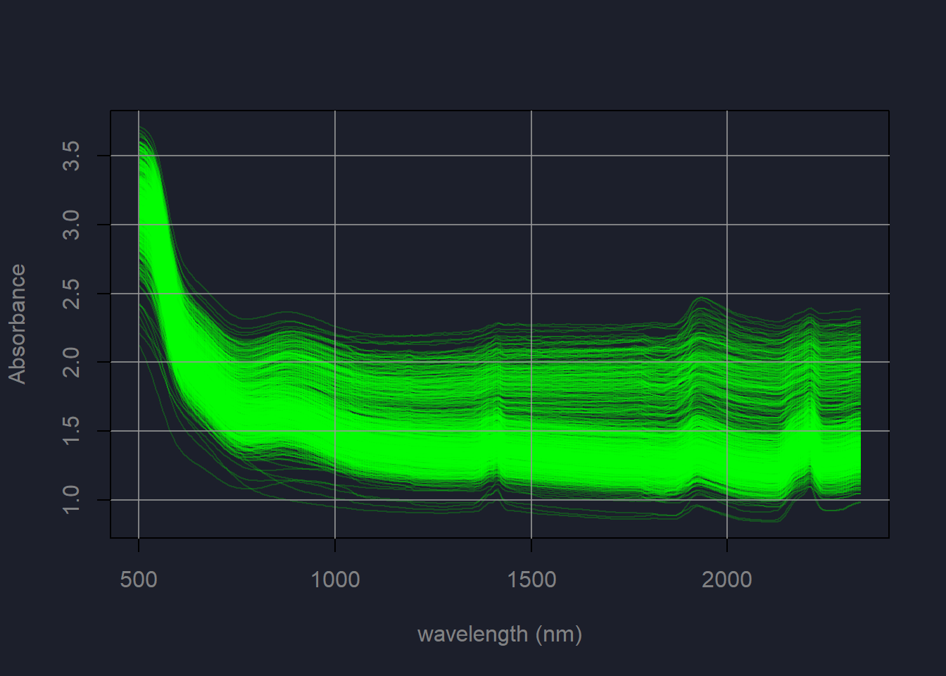
Figure 3.1: Spectra in the SoilNIRSaoPaulo dataset
## reset the background color of your plots to the original color
par(bg = obg)
In addition you also need a R object of class (SpatialPolygonsDataFrame of the package sp) which contains the polygon of the study area. You can also download the file (polygon.rds) containing this object by clicking here.